Running MiSSE

Background

In Beaulieu and O’Meara (2016) we pointed out that the trait-independent HiSSE model is basically a model for traits and a separate model for shifts in diversification parameters, much like BAMM (though without priors, discontinuous inheritance of extinction probability, or other mathematical foibles). The hidden states can drive different diversification processes, and the traits just evolve under a regular Markovian trait model. At that point, there is no harm in just dropping the trait altogether and just focusing on diversification driven by unknown factors. This is what we meant by our HiSSE framework essentially forming a continuum from a purely trait-independent model (e.g., BAMM, or MEDUSA), to a completely trait-dependent model (e.g., BiSSE)(see discussion in Caetano et al., 2018). That is what this MiSSE function does – it sets up and executes a completely trait-free version of a HiSSE model. Thus, all that is required is a tree. The model allows up to 26 possible hidden states in diversification (denoted by A-Z). Transitions among hidden states are governed by a single global transition rate, \(q\). A “shift” in diversification denotes a lineage tracking some unobserved, hidden state. An interesting byproduct of this assumption is that distantly related clades can actually share the same discrete set of diversification parameters.

Note that we refer to “hidden state” simply as a shorthand. We do not mean that there is a single, discrete character that is solely driving diversification differences. There is some heritable “thing” that affects rates, such as a combination of body size, oxygen concentration, trophic level, and, say, how many total species are competing for resources in an area. In other words, it could be that there is some single discrete trait that drives everything. However, it is more likely that a whole range of factors play a role, and we just slice them up into discrete categories, the same way we slice up mammals into carnivore / omnivore / herbivore or plants into woody / herbaceous when the reality is more continuous. This is true for HiSSE, but this concept is especially important to grasp for MiSSE.

Setting up a MiSSE model

The set up is similar to other functions in hisse, except there is no need to set up a transition model For the following example, we will use the cetacean phylogeny (e.g., whales and relatives) of Steeman et al. (2009).

suppressWarnings(library(hisse))

## Loading required package: ape

## Loading required package: deSolve

## Loading required package: GenSA

## Loading required package: subplex

## Loading required package: nloptr

phy <- read.tree("whales_Steemanetal2009.tre")

As with hisse, rather than optimizing \(\lambda_i\) and \(\mu_i\) separately, MiSSE optimizes transformations of these variables. We let \(\tau_i = \lambda_i+\mu_i\) define “net turnover”, and we let \(\epsilon_i = \mu_i / \lambda_i\) define the “extinction fraction”. This reparameterization alleviates problems associated with over-fitting when \(\lambda_i\) and \(\mu_i\) are highly correlated, but both matter in explaining the diversity pattern (see discussion of this issue in Beaulieu and O’Meara 2016). The number of free parameters in the model for both net turnover and extinction fraction are specified as index vectors provided to the function call. First, let us fit a single rate model:

turnover <- c(1)
eps <- c(1)
one.rate <- MiSSE(phy, f=1, turnover=turnover, eps=eps)

Pretty simple. Now to fit a model that contains two rate classes, we will simply expand out the turnover vector:

turnover <- c(1,2)
eps <- c(1,1)
two.rate <- MiSSE(phy, f=1, turnover=turnover, eps=eps)

Overall, MiSSE allows up to 26 possible hidden states in diversification (denoted by A-Z), and in this example since we fit two rate classes, we have two hidden states, A and B, impacting turnover rates. Here is the rest of the model set applied to the whale data set:

#rate classes A:C
turnover <- c(1,2,3)
eps <- c(1,1,1)
three.rate <- MiSSE(phy, f=1, turnover=turnover, eps=eps)
#rate classes A:D
turnover <- c(1,2,3,4)
eps <- c(1,1,1,1)
four.rate <- MiSSE(phy, f=1, turnover=turnover, eps=eps)
#rate classes A:E
turnover <- c(1,2,3,4,5)
eps <- c(1,1,1,1,1)
five.rate <- MiSSE(phy, f=1, turnover=turnover, eps=eps)

We can also let \(\epsilon_i\) vary across the tree:

turnover <- c(1,2)
eps <- c(1,2)
two.rate.weps <- MiSSE(phy, f=1, turnover=turnover, eps=eps)

#rate classes A:C, but include eps as well:
turnover <- c(1,2,3)
eps <- c(1,2,3)
three.rate.weps <- MiSSE(phy, f=1, turnover=turnover, eps=eps)

However, in the case of cetaceans, allowing extinction fraction to vary does not provide any additional information to the model as all rate classes return nearly identical estimates (not shown).

I have already fit these models. Figure 1 shows the improvement in AIC as we increase the complexity of the model.

The fit of an incremental increase in the number of rate classes estimated under a MiSSE analysis of the cetacean phylogeny of Steeman et al. (2009). There is a clear reduction in AIC from one to three rate classes, which levels off at four rate classes and five rate classes returns an AIC that is about 1 unit higher than either the three and four rate class.

##Plotting MiSSE reconstructions

Like with all other functions, we provide plotting functionality with plot.misse.states() for hidden state reconstructions of class misse.states output by our MarginReconMiSSE() function. And, as with other functions, a single misse.states object can be supplied and the plotting function will provide a heat map of the diversification rate parameter of choice, or a list of misse.states objects can be supplied and the function will “model-average” the results. For plotting rates, users can choose among turnover, net diversification (“net.div”), speciation, extinction, or extinction fraction (“extinction.fraction”). Below is an example of how to run the reconstruction function to obtain misse.states output from our two rate model for cetaceans. But, again, for simplicity, I have a file that contains the reconstructions and we can check that everything has loaded correctly and is of the proper misse.states class:

# two.rate.recon <- MarginReconMiSSE(phy=phy, f=1,  hidden.states=2, 
                #pars=two.rate$solution, n.cores=3, AIC=two.rate$AIC)
load("misse.vignette.Rsave") # Line above shows the command to create this result.
class(two.rate.recon)

## [1] "misse.states"

two.rate.recon

## 
## Phylogenetic tree with 87 tips and 86 internal nodes.
## 
## Tip labels:
##   Balaena_mysticetus, Eubalaena_australis, Eubalaena_glacialis, Eubalaena_japonica, Caperea_marginata, Eschrichtius_robustus, ...
## Node labels:
##   1, 1, 1, 1, 1, 1, ...
## 
## Rooted; includes branch lengths.

Let’s take a look at the reconstruction for the two.rate model reconstruction. I will simply supply the reconstruction object if misse.states class to the plotting function, plot.misse.states(), and plot net diversification (see Figure 2).

plot.misse.states(two.rate.recon, rate.param="net.div", show.tip.label=TRUE, type="phylogram",
                  fsize=.25, legend="none")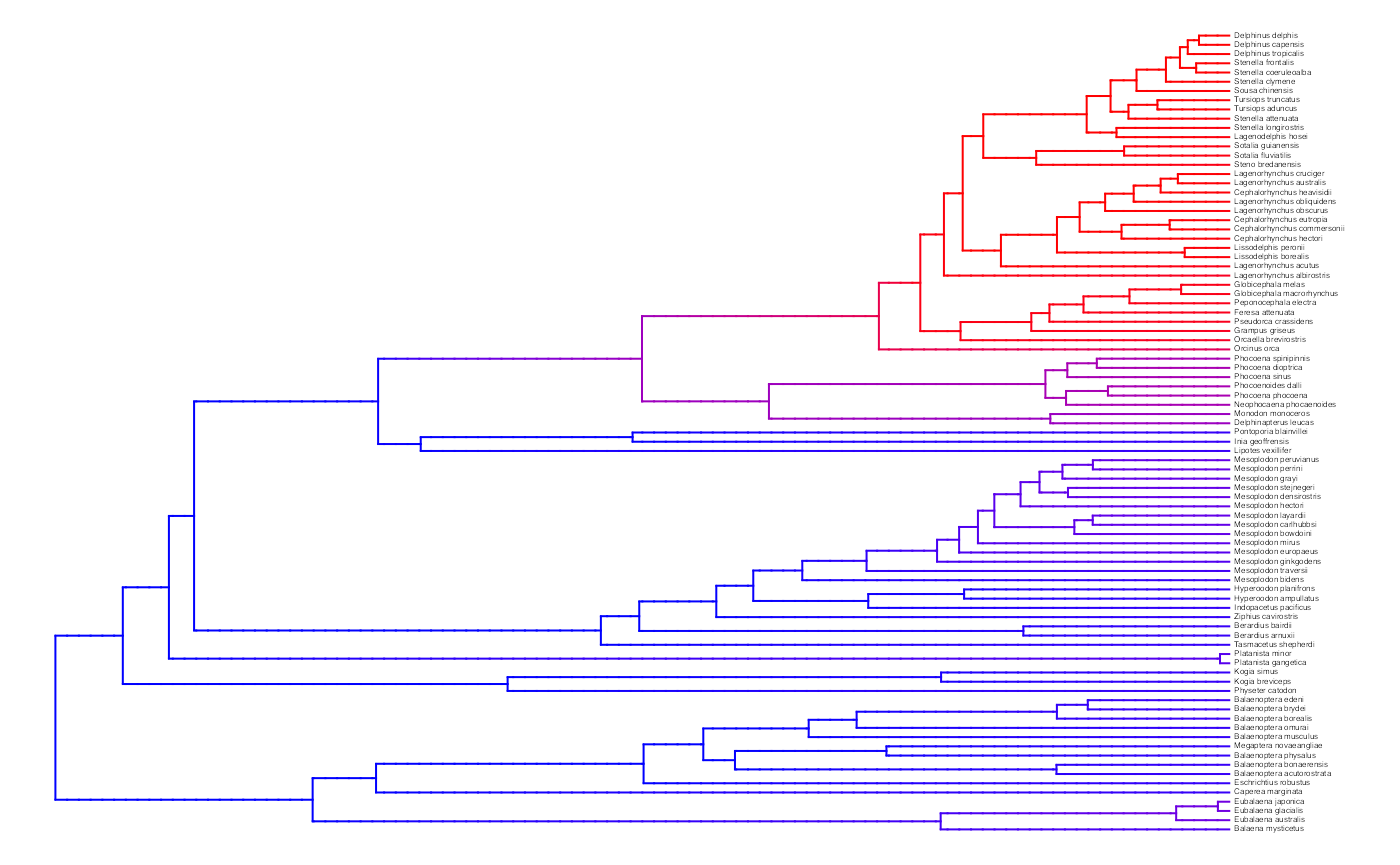

A two-rate class MiSSE analysis and reconstruction of the cetacean phylogeny of Steeman et al. (2009) shows a clear increase in the net diversification rate within the Delphinidae (dolphins) relative to all other cetaceans; there also seems to be a slightly elevated rates in the sister group of Delphinidae, the Monodontidae+Phocenidae. Overall, this particular MiSSE model seems to correctly identify the source of ‘trait-independent’ diversification that can plague BiSSE analyses of simulated data sets on the cetacean tree (see Rabosky and Goldberg, 2015).

## $rate.tree
## Object of class "contMap" containing:
## 
## (1) A phylogenetic tree with 87 tips and 86 internal nodes.
## 
## (2) A mapped continuous trait on the range (0.074823, 0.205397).

Of course, in this example we have a set of models that includes models that contain upwards of five rate classes. Also, we know from AIC that there are three model – the three-, four-, and five rate class models – that are within 2 AIC units away from each. As we do in all other hisse functions, we allow for plots to be model-averaging of the rates at nodes and tips. To do this, we simply supply all reconstructions you want to average as elements in a list. There are many ways to generate a list, but here is one way:

misse.results.list = list()
misse.results.list[[1]] = one.rate.recon
misse.results.list[[2]] = two.rate.recon
misse.results.list[[3]] = three.rate.recon
misse.results.list[[4]] = four.rate.recon
misse.results.list[[5]] = five.rate.recon

And, as before, we simply supply this list to the plotting function, plot.misse.states(), and plot net diversification (see Figure 3).

plot.misse.states(misse.results.list, rate.param="net.div", show.tip.label=TRUE, type="phylogram",
                  fsize=.25, legend="none")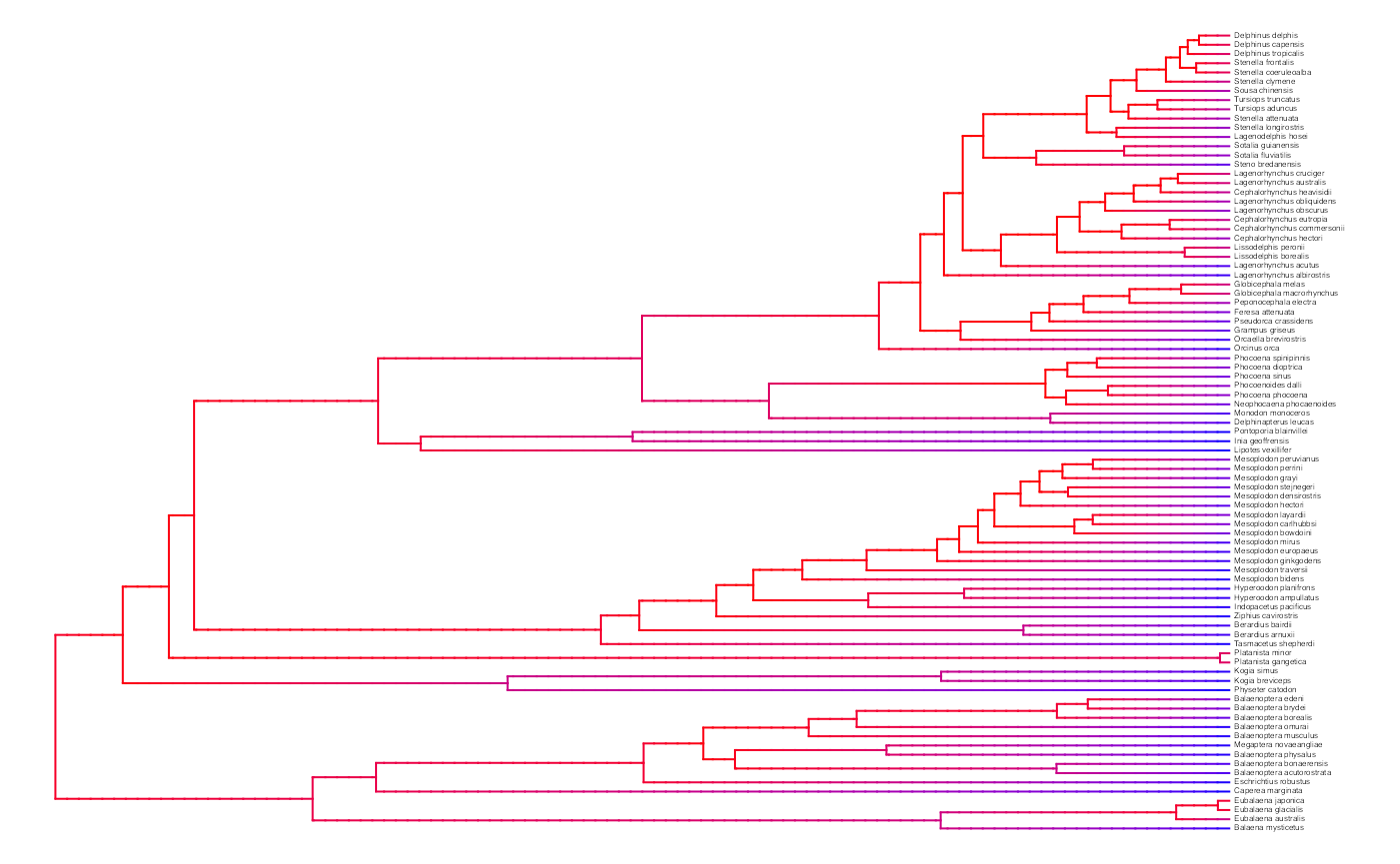

A model-averaged MiSSE analysis of the cetacean phylogeny of Steeman et al. (2009) shows an apparent slow down in the net diversification through time.

## $rate.tree
## Object of class "contMap" containing:
## 
## (1) A phylogenetic tree with 87 tips and 86 internal nodes.
## 
## (2) A mapped continuous trait on the range (0.047889, 0.229038).

Fixing extinction fraction

Estimating extinction is hard. This affects all diversification models (even if all you want and look at is speciation rate, extinction rate estimates still affect what this is as they affect the likelihood). It is most noticeable in MiSSE with extinction fraction (extinction rate divided by speciation rate). One option, following Magallon & Sanderson (2001), is to set extinction fraction at set values. We have made this straightforward to do in the MiSSE() function call. The first step is to setup a Yule-based MiSSE() run by supplying a vector of zeros for eps that is of equal length to the number of turnover rate classes:

turnover <- c(1,2)
eps <- c(0,0)

In the function call, there is an option called fixed.eps. Normally, this is set to NULL, which indicates that extinction fraction is to be estimated. When a value is supplied to fixed.eps this will be the value used throughout the parameter search. Here we assume there are two rate classes and a fixed extinction fraction of 0.90:

two.rate <- MiSSE(phy, f=1, turnover=turnover, eps=eps, fixed.eps=0.9)

Other considerations

Like with hisse, GeoHiSSE, and MuHiSSE, there are functions available for generating estimates of the uncertainty in the parameter estimates (i.e., SupportRegionMiSSE()), and to obtain model averages (i.e., GetModelAveRates()) for nodes, for tips, or for both to be used in post-hoc tests. Users are encouraged to read other vignettes and help pages provided for more information. For more conceptual discussions of these functions and ideas, readers are also encouraged to read Caetano et al. (2018).

There are two additional items that are worth mentioning. First, like with MuHiSSE, I would recommend users try multiple random starting points when optimizing any given model with MiSSE. In Nakov et al. (2018), we found that the default starting values often did not return the highest log likelihood. To alleviate this issue, we performed \(\ge\) 50 maximum likelihood optimizations for each model, each initiated from a distinct starting point. All functions within hisse are provided with starting.vals option for these purposes.

Second, we note that MiSSE may seem slower than most other functions within hisse. This is somewhat intentional. Underneath the hood we have implemented a lot of checks to the integration for calculating probabilities along branches. This will mean that often times weird messages will spit out to the screen. For now, ignore them, the optimization “feels” these issues and takes necessary action. But this also means that users must pay particular attention to the complexity of the models they are fitting and critically think whether or not the parameters make sense. For example, in cetacean tree used above, I attemped to fit a model with three, four, and five hidden states, A, B, and C, but the reconstructions indicated a rather complicated, and highly uncertain, diversification history:

two.rate

## 
## Fit 
##             lnL             AIC            AICc          n.taxa n.hidden.states 
##       -271.7681        551.5363        552.0241         87.0000          2.0000 
## 
## Model parameters: 
## 
##   turnover0A        eps0A   turnover0B        eps0B           q0 
## 7.489769e-02 2.061154e-09 2.052022e-01 2.061154e-09 3.743782e-03

three.rate

## 
## Fit 
##             lnL             AIC            AICc          n.taxa n.hidden.states 
##       -263.9931        537.9863        538.7270         87.0000          3.0000 
## 
## Model parameters: 
## 
##  turnover0A       eps0A  turnover0B       eps0B  turnover0C       eps0C 
## 0.008069096 0.275802793 0.008083110 0.275802793 0.340152955 0.275802793 
##          q0 
## 0.131447160

Note that the likelihood was a significant improvement from the two rate model, but the transition rate, \(q\), is roughly two orders of magnitude higher (\(q=0.131\)) relative to the two-rate model estimate (\(q=0.004\)). The same is true for the four and five rate class models. What does this mean? Well, we can convert this into the expected number of transitions by multiplying the rate by the sum of the branch lengths in the cetacean phylogeny:

expected.transitions.two <- 0.004 * sum(two.rate$phy$edge.length)
expected.transitions.two

## [1] 3.281109

expected.transitions.three <- 0.131 * sum(three.rate$phy$edge.length)
expected.transitions.three

## [1] 107.4563

At first glance, this might seem that something is off with the three-rate class model – e.g., 3 vs. 107 number of shifts among the different classes? However, examining the support region around the parameters can give an indication as to the overall reliability of these estimates:

load("misse.support.Rsave")
two.rate.support$ci[,"q0"]

##           0%          25%          50%          75%         100% 
## 0.0009535839 0.0036835840 0.0065180114 0.0106515654 0.0206332391

three.rate.support$ci[,"q0"]

##         0%        25%        50%        75%       100% 
## 0.06839226 0.11308939 0.13144716 0.15736921 0.22772718

In the case of the two rate class model, even though the MLE indicates very few transitions among the rate classes, there is a model within 2 log likelihood units that suggests as many as 17 expected transitions. In other words, the \(q\) estimate even under the two rate class model is fairly certain. We suspect that what is being picked up by these models is something that is both clade-specific (i.e., implied by the two rate class model) and time-dependent (i.e., implied by the three, four, and five rate class models), with the latter exerting the strongest influence on the overall fit.

MiSSE Greedy

With the way MiSSE() is implemented there are 52 possible models one could try, which would require coding each model by hand. Of course, a model where there are 26 different classes of turnover rates may be far too parameter rich that it’s not even worth trying. The difficulty then is determining what the “right” stopping point is in terms of adding further model complexity. We implemented MiSSEGreedy() as means of automating the process of fitting a set of MiSSE() models. It first runs a chunk of models, determines the “best” based on AIC, then it continues on from that complexity until the a more complex model is less than some user defined \(\Delta\)AIC than the current best model. At that point, MiSSEGreedy() stops running new models. Since this is based on current best AICc, and we start with simplest models. However, note that this produces an asymmetry, where a terrible model with no rate variation is always included, but a slightly less terrible model with 26 turnover rates might never be evaluated.

This functions work much faster when run in parallel. To do this, we include an option n.cores to allow users to set the number of available cores on your machine. The default is one core. Since many models are evaluated, the most natural approach is to run one model per core, see if at least one of the models are still ok, then send out the next models out to all the cores. Setting n.cores to the number of parallel jobs you want, and leaving chunk.size set to NULL, will do this. However, this is slightly inefficient – the odds are that some cores will finish earlier than others, and will be waiting until all finish. So a different approach is to set a chunk.size greater than n.cores – it will still use no more than n.cores at a time, but once one model in the set finishes it will send off the next until all models in the chunk are run. This keeps the computer even busier, but then it won’t stop to check to make sure the models are still feasible as often, and it only saves intermediate results after each chunk of models finishes. Our recommendation is to use n.cores=parallel::detectCores() if you’re on a machine where you can use all the cores and leave chunk.size unspecified (so it will also default to n.cores), but it’s up to you.

After every chunk of models are done, this function will display the status: what models have been run, what the likelihoods and AICs are, etc. It will also predict how long future runs will check, based on a linear regression between the number of free parameters and log(minutes to run). These are just estimates based on the runs so far, but it’s a stochastic search and can take more or less time. Here is a very straightforward MiSSEGreedy() run:

tree <- rcoal(50)
potential.combos <- generateMiSSEGreedyCombinations(max.param=4, vary.both=TRUE)

#run on one core:
model.set <- MiSSEGreedy(tree, possible.combos=potential.combos, n.cores=1)

#run on all available cores: (commented out because CRAN does not allow this in examples)
model.set <- MiSSEGreedy(phy, potential.combos, n.cores=parallel::detectCores(), f=1)

AICc <- unlist(lapply(result, "[[", "AICc"))
deltaAICc <- AICc-min(AICc)
print(length(result))

# Yes, [[ is a function you can lapply, and the name of elements within each list
# object can be arguments. Life is awesome.

The output in model.set is a list of models evaluated. From there you can just loop over each model and do the rate class reconstruction:

model.recons <- as.list(1:length(model.set))
for (model_index in 1:length(model.set)) {
    nturnover <- length(unique(model.set[[model_index]]$turnover))
    neps <- length(unique(model.set[[model_index]]$eps))
    misse_recon <- MarginReconMiSSE(phy = model.set[[model_index]]$phy, f = 1, 
                                    hidden.states = nturnover, 
                                    pars = model.set[[model_index]]$solution, 
                                    AIC = model.set[[model_index]]$AIC)
    model.recons[[model_index]] <- misse_recon
}

As with any other function contained within hisse, the output from the character reconstruction can be used to obtain model averaged rates, such the estimated rates for each tip in the tree:

tip.rates <- GetModelAveRates(model.recons, type = c("tips"))

We recommend also taking a look at the function generateMiSSEFGreedyCombinations(), which we used in the MiSSEGreedy() example above. This creates the set of combinations of models to run through MiSSEGreedy() as a data.frame. It has columns for the number of rates to estimate for turnover, the number of values to estimate for extinction fraction (eps), and any fixed values for eps to apply to the whole tree. You can add your own rows or delete some to this data.frame to add more or fewer combinations. By default, this comes out ordered so that simpler models are run first in MiSSEGreedy() but that is not required (but wise for most use cases), and you can reorder if you wish. turnover.tries and eps.tries set how many turnover and eps hidden states to try, respectively. If you wanted to try only 1, 3, and 7 hidden states for turnover you would set turnover.tries = c(1, 3, 7) for example.

As discussed above estimating extinction rates is hard. This affects all diversification models (even if all you want and look at is speciation rate, extinction rate estimates still affect what this is as they affect the likelihood). It is most noticeable in MiSSE with eps, the extinction fraction (extinction rate divided by speciation rate). One option, following Magallon & Sanderson (2001), is to set extinction fraction at set values. By default, we use the somewhat arbitrary values of Magallon & Sanderson (2001) – 0 (meaning a Yule model - no extinction) or 0.9 (a lot of extinction, though still less than paleontoligists find). You can set your own in fixed.eps.tries. If you only want to use fixed values, and not estimate, get rid of the NA, as well. However, don’t “cheat” – if you use a range of values for fixed.eps, it’s basically doing a search for this, though the default AICc calculation doesn’t “know” this to penalize it for another parameter.

HiSSE and, by extension, MiSSE assume that a taxon has a particular hidden state. Thus, they’re written to assume that we “paint” these states on the tree and a given state affects both turnover and eps. So if turnover has four hidden states, eps has four hidden states. They can be constrained: the easiest way is to have, say, turnover having an independent rate for each hidden state and eps having the same rate for all the hidden states. If vary.both is set to FALSE, all models are of this sort: if turnover varies, eps is constant across all hidden states, or vice versa. Jeremy Beaulieu prefers this. If vary.both is set to TRUE, both can vary: for example, there could be five hidden states for both turnover and eps, but turnover lets each of these have a different rate, but eps only allows three values (so that eps_A and eps_D might be forced to be equal, and eps_B and eps_E might be forced to be equal). Brian O’Meara would consider allowing this, while cautioning you about the risks of too many parameters.

References

Beaulieu, J.M., and B.C. O’Meara. (2016). Detecting hidden diversification shifts in models of trait-dependent speciation and extinction. Syst. Biol. 65:583-601.

Caetano, D.S., B.C. O’Meara, and J.M. Beaulieu. (2018). Hidden state models improve state-dependent diversification approaches, including biogeographic models. Evolution, 72:2308-2324.

Magallón, S, and M.J. Sanderson. (2001). Absolute diversification rates in angiosperm clades. Evolution 55:1762-1780.

Nakov, T., J.M. Beaulieu, and A.J. Alverson. (2018). Freshwater diatoms diversify faster than marine in both planktonic and benthic habitats. bioRxiv, doi: https://doi.org/10.1101/406165.

Rabosky, D.L., and E.E. Goldberg. (2015). Model inadequacy and mistaken inferences of trait-dependent speciation. Syst. Biol. 64:340-355.